20190221

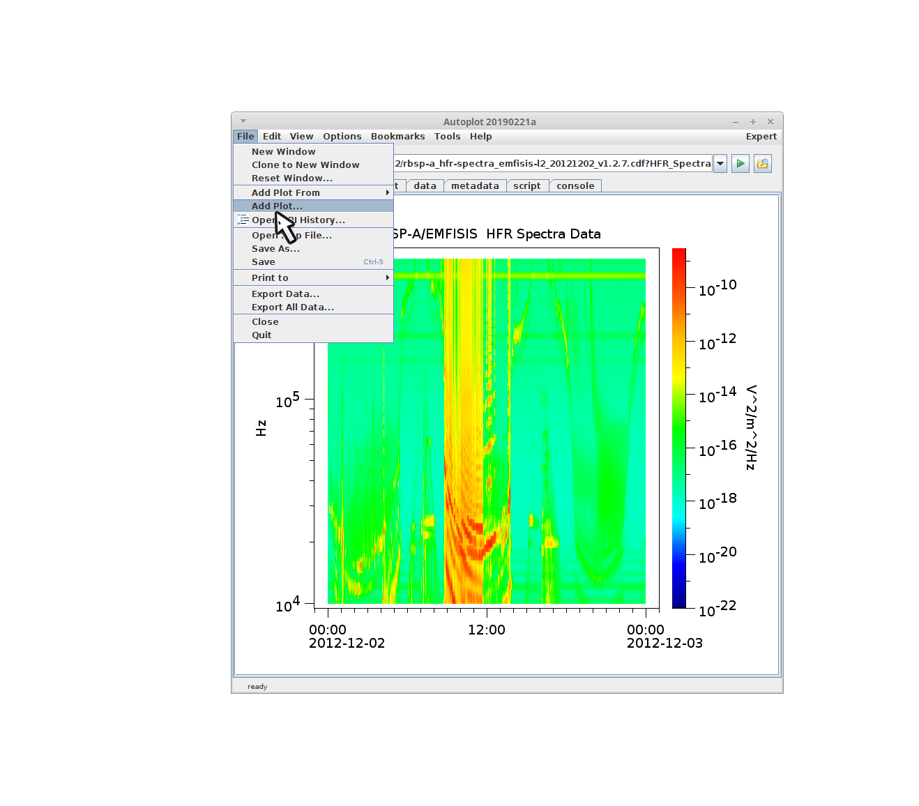
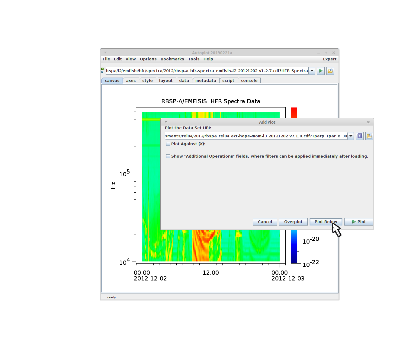
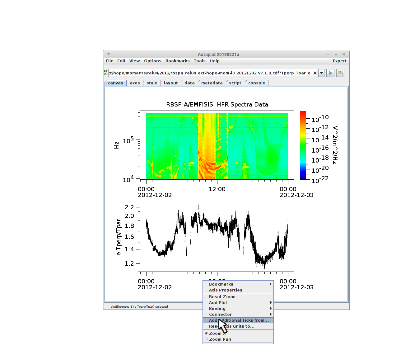
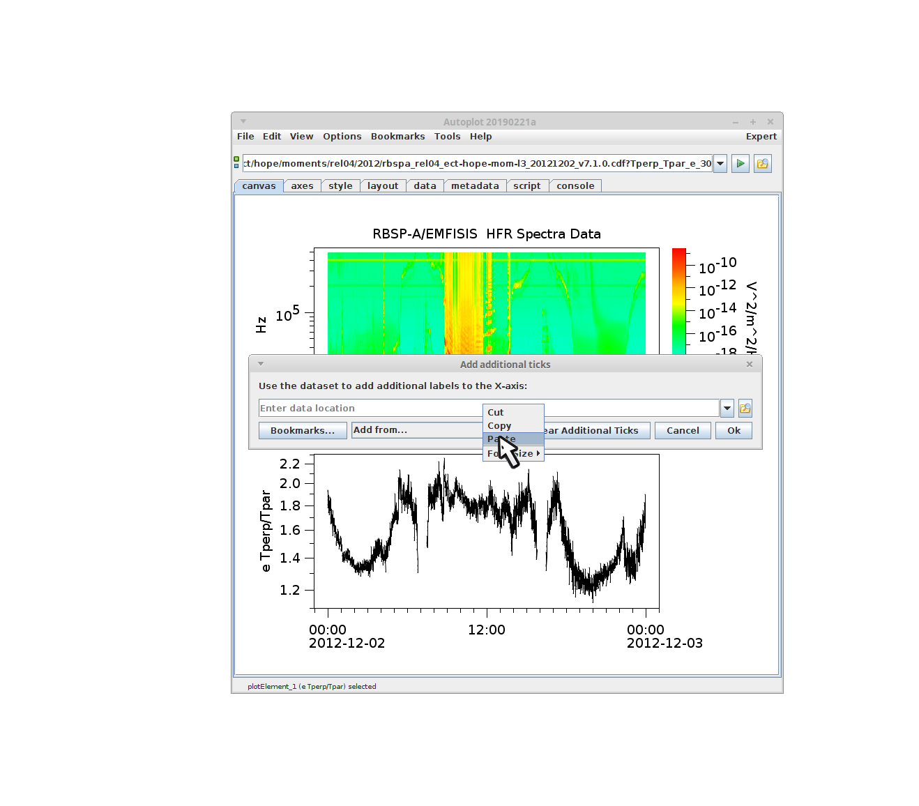
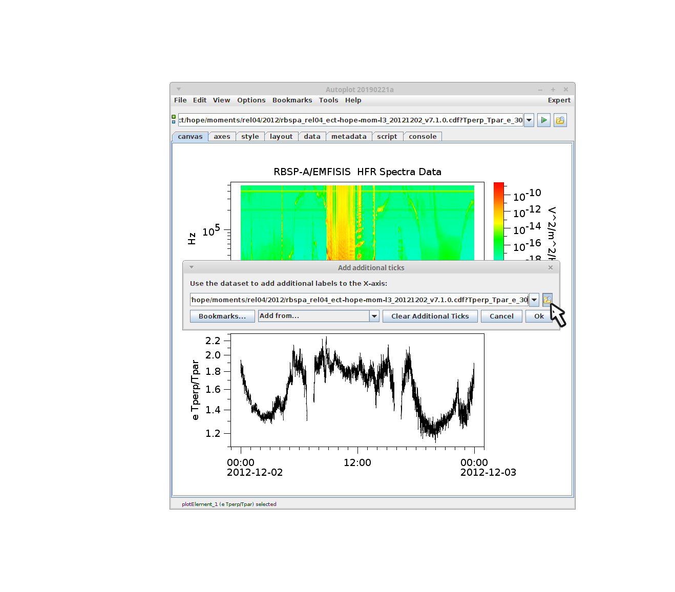
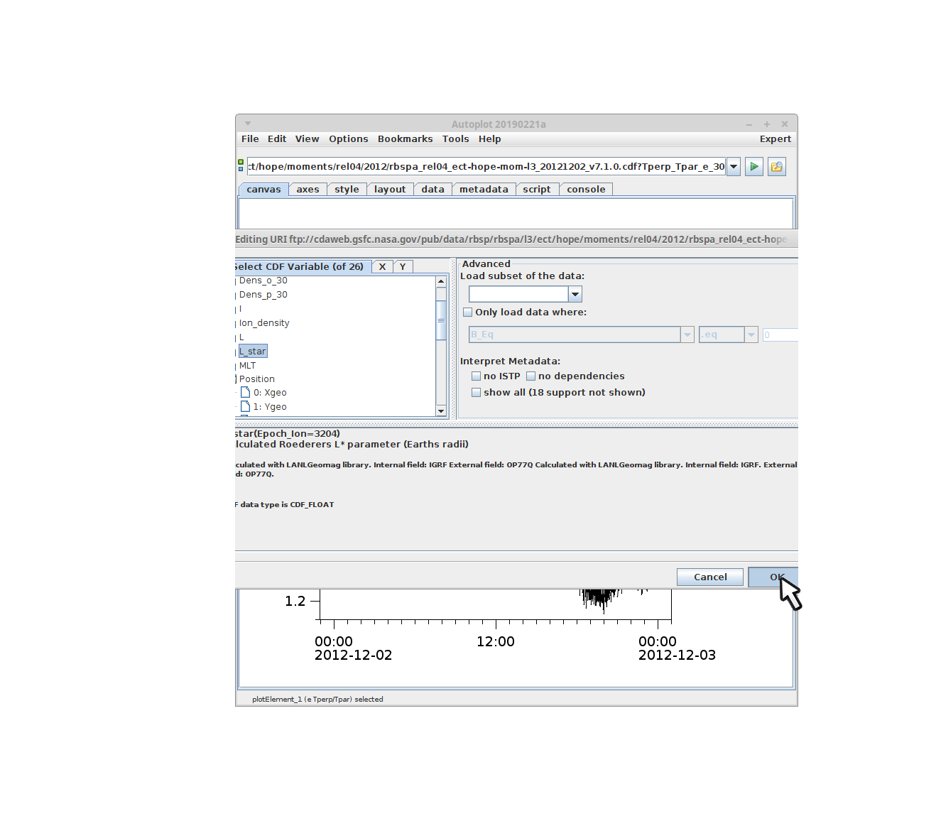
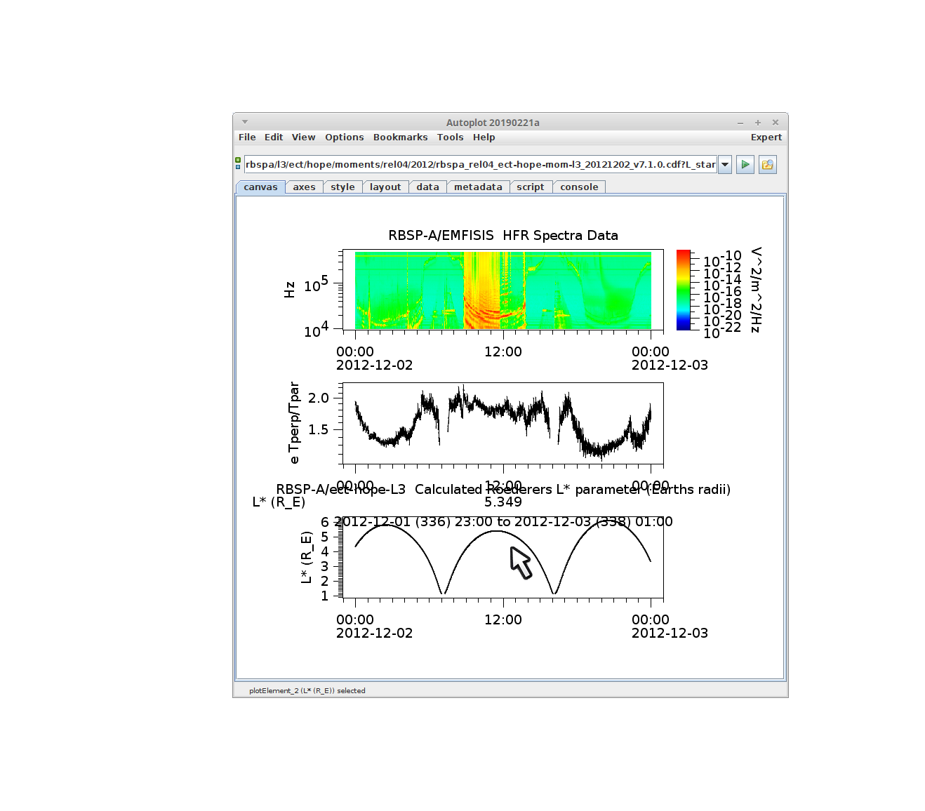
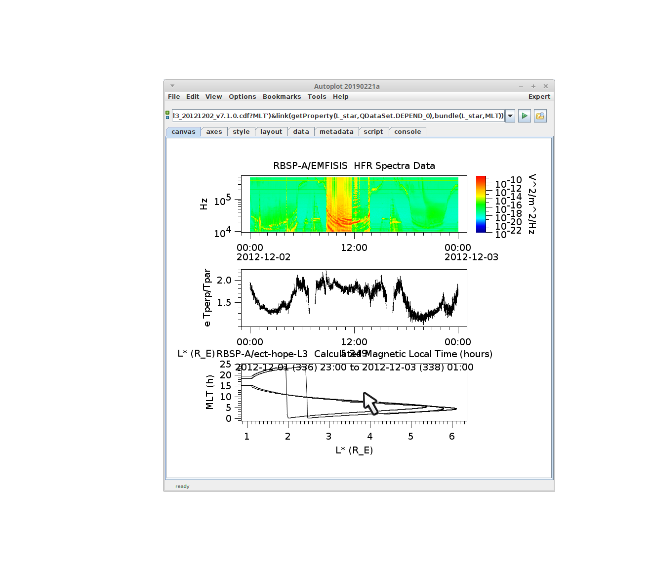
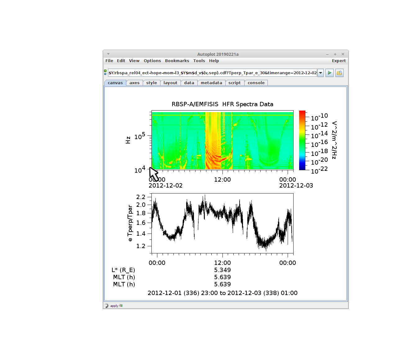
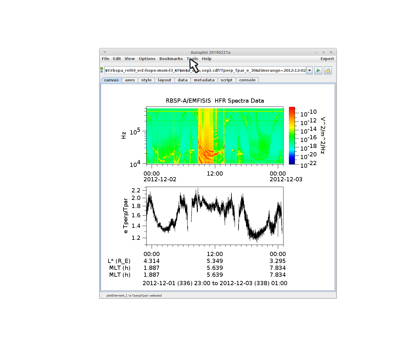
Scott asks: How to use autoplot to load ftp://cdaweb.gsfc.nasa.gov/pub/data/rbsp/rbspa/l2/emfisis/hfr/spectra/2012/rbsp-a_hfr-spectra_emfisis-l2_20121202_v1.2.7.cdf?HFR_Spectra, and for the lower panelftp://cdaweb.gsfc.nasa.gov/pub/data/rbsp/rbspa/l3/ect/hope/moments/rel04/2012/rbspa_rel04_ect-hope-mom-l3_20121202_v7.1.0.cdf?Tperp_Tpar_e_3 and then ephemeris ticks L*, MLat, MLT

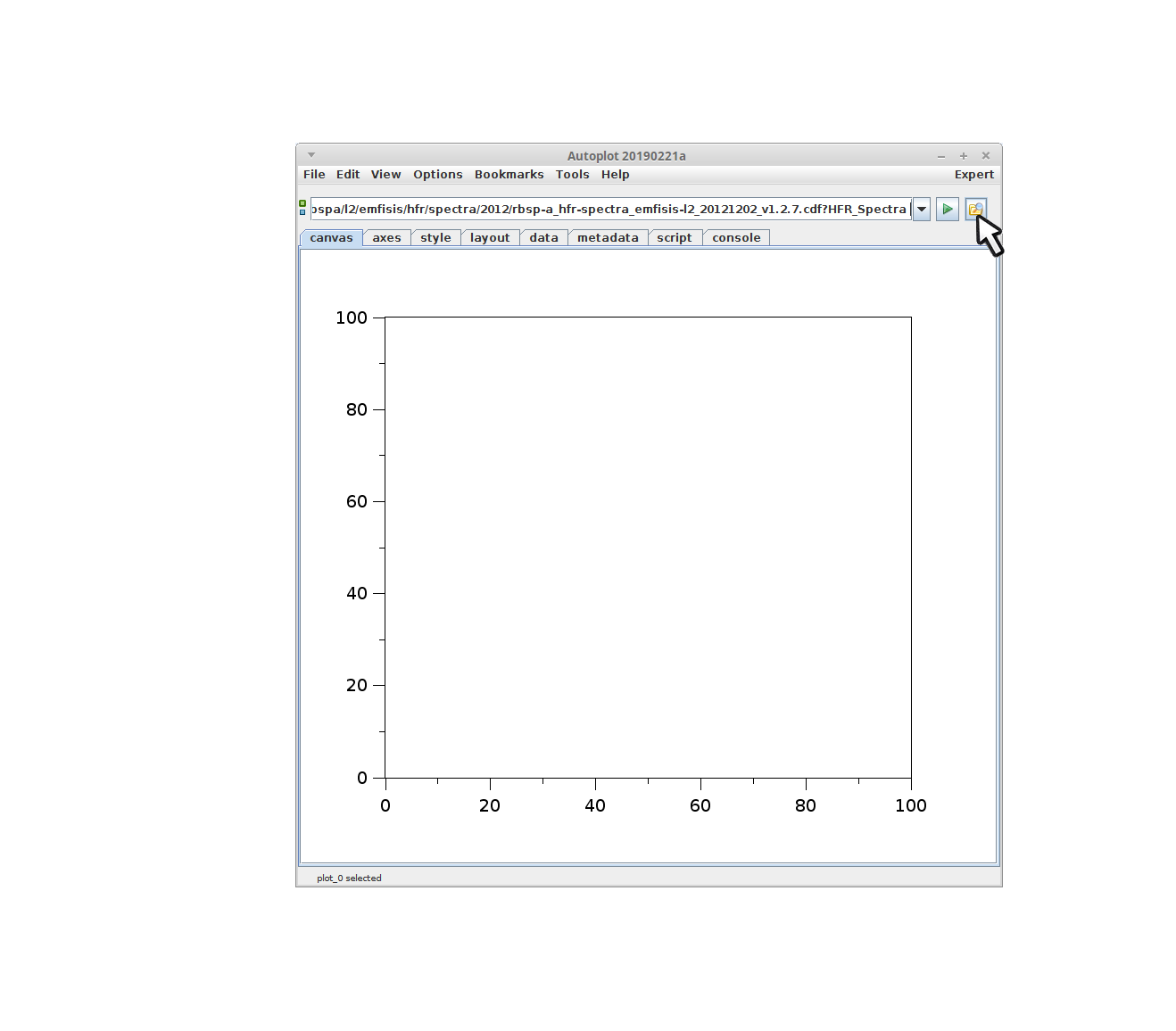
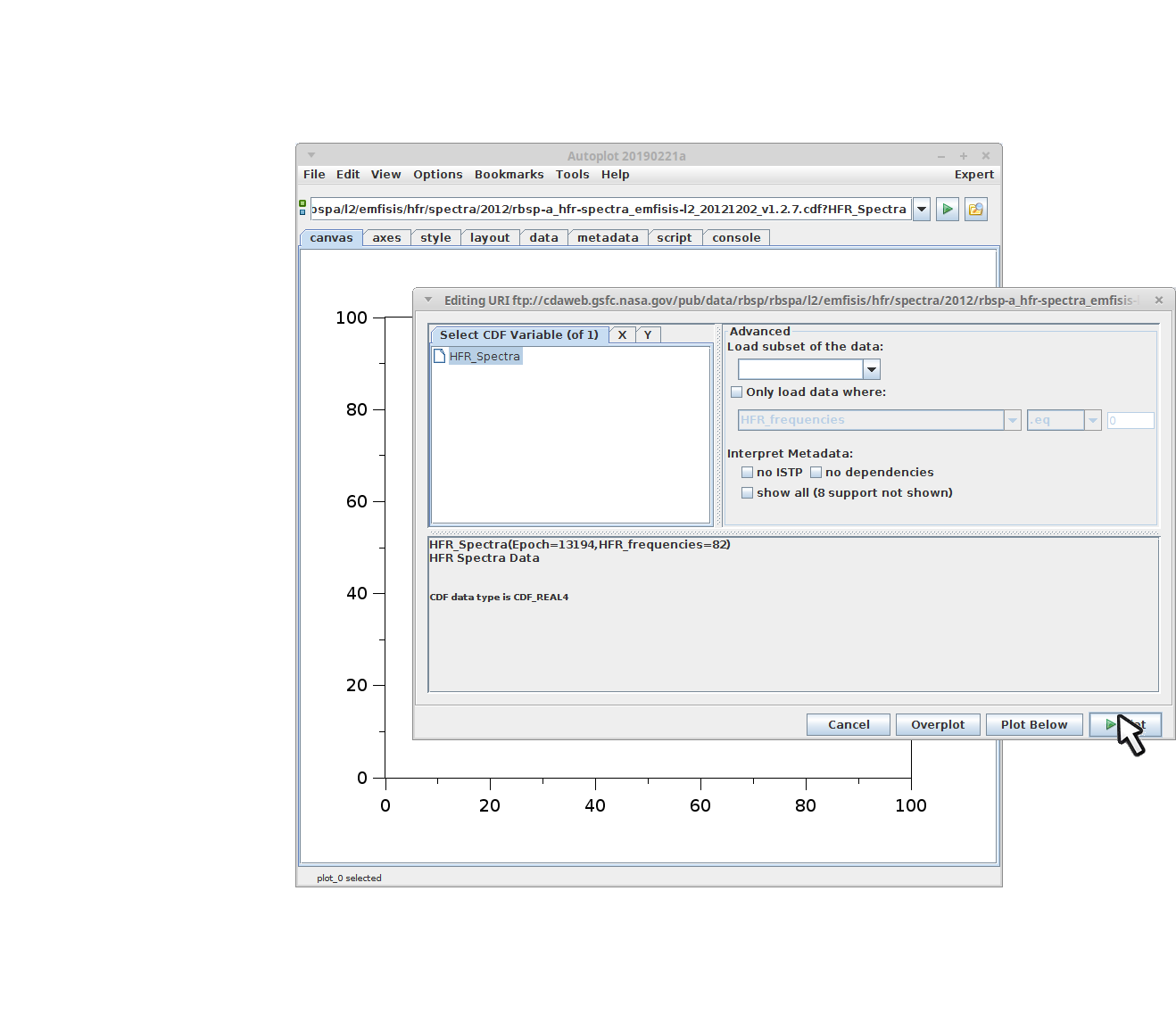
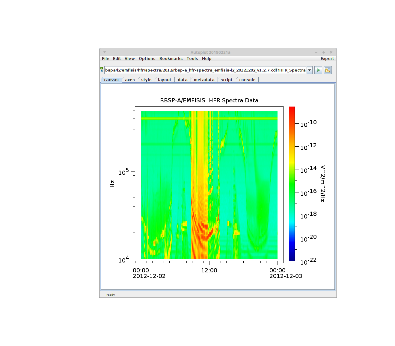
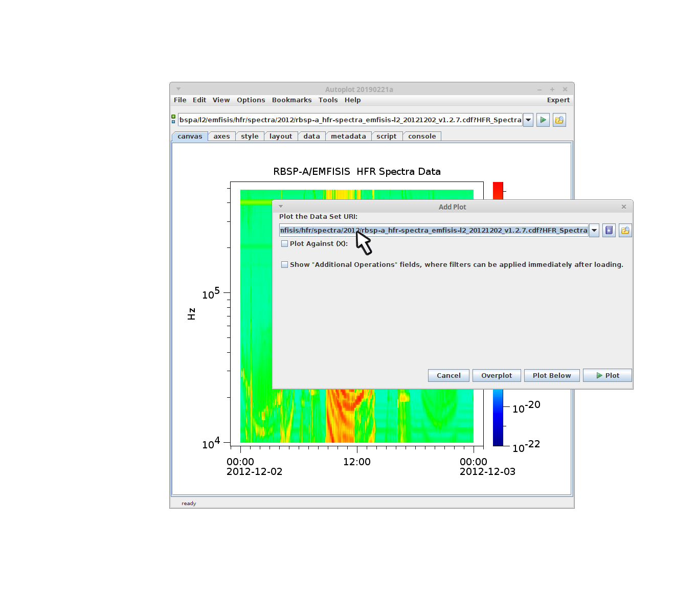
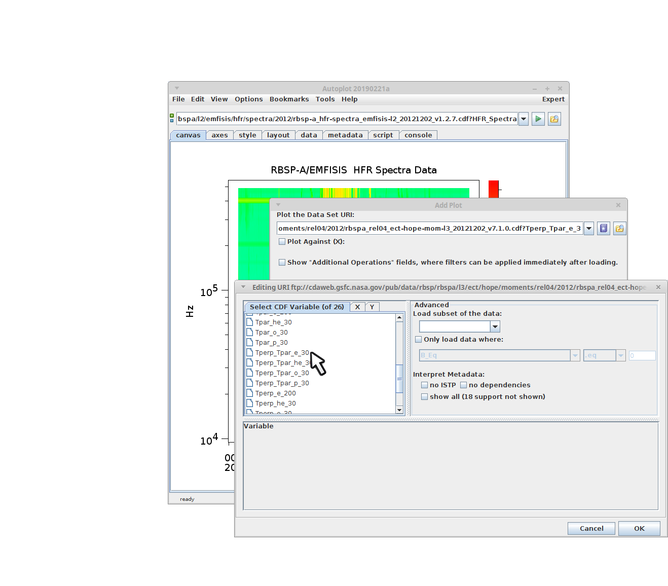
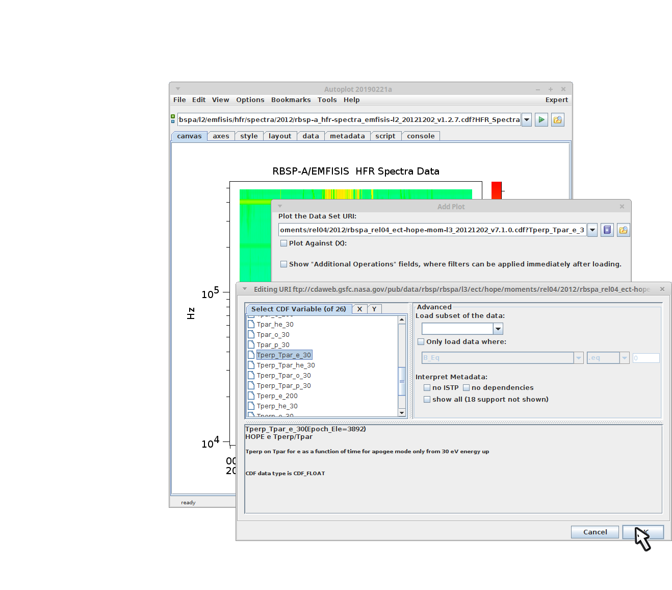
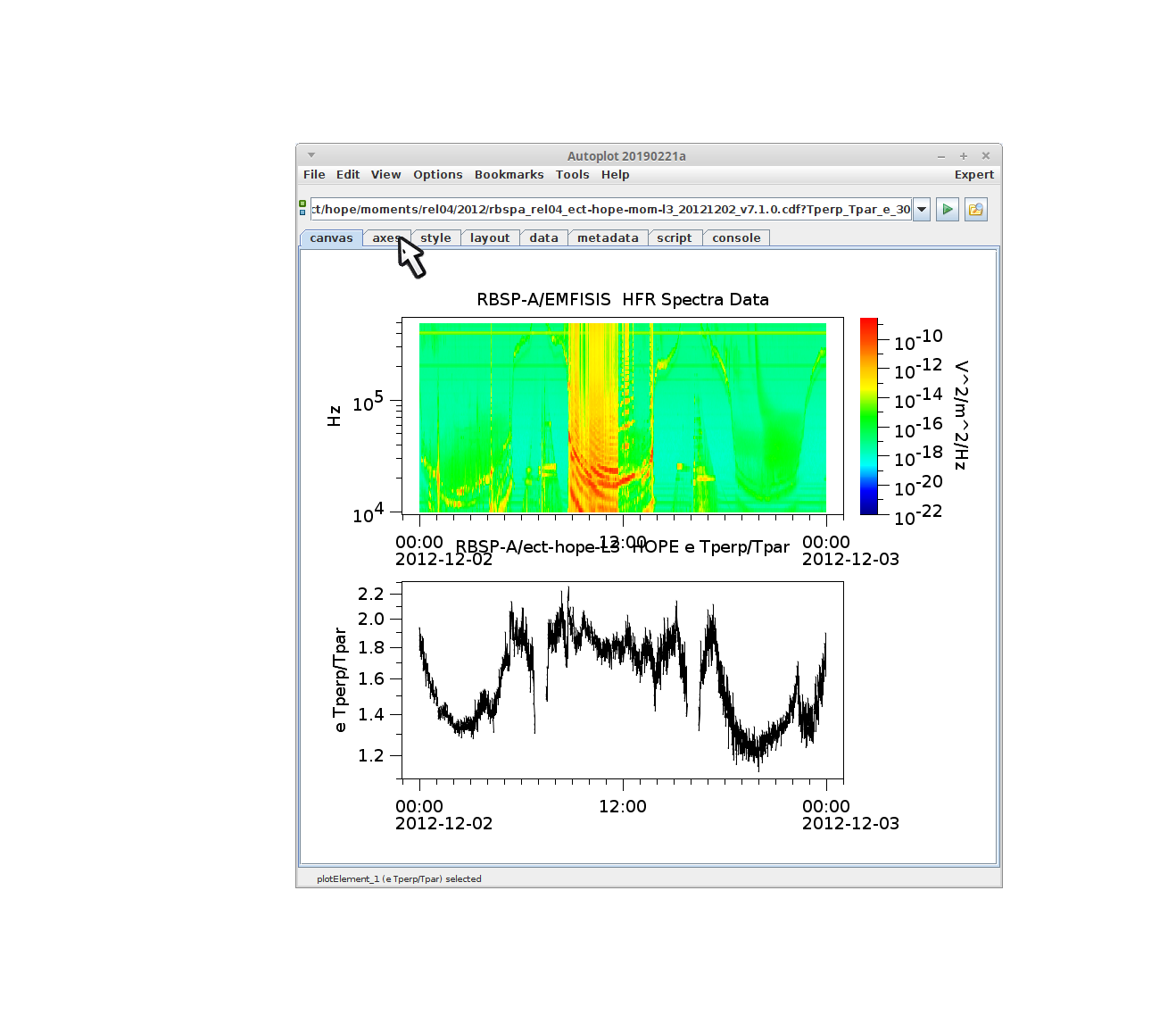
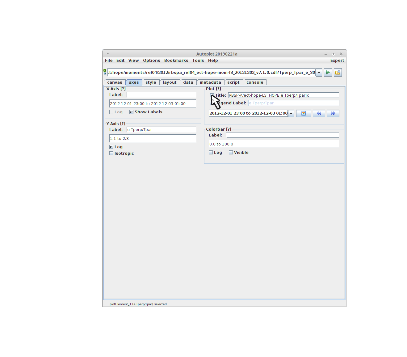
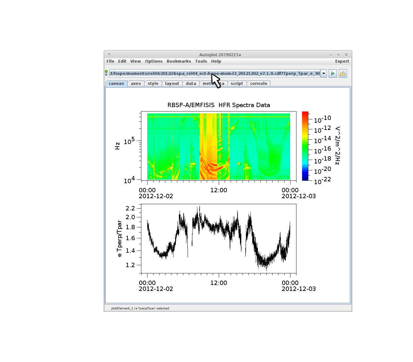
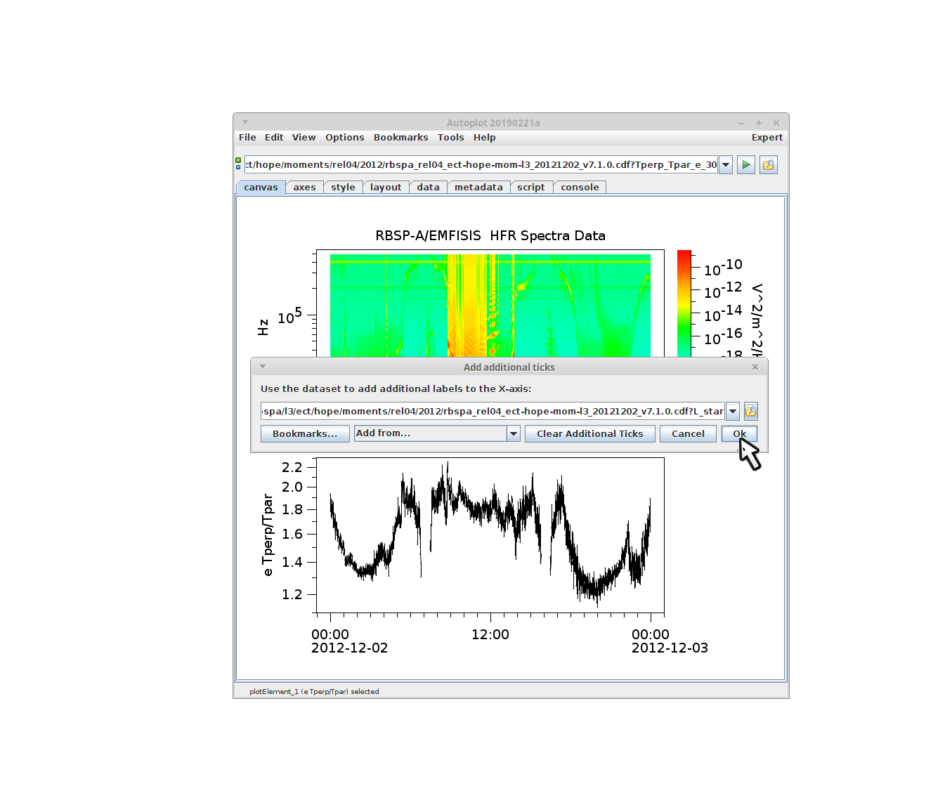
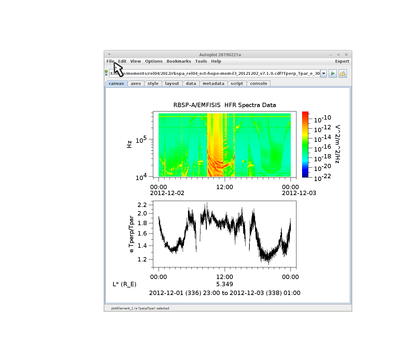
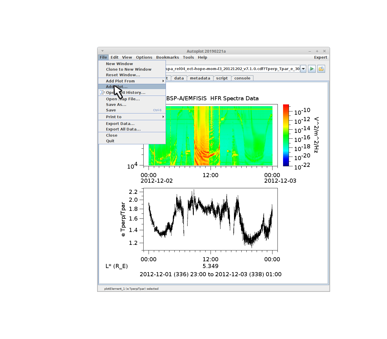
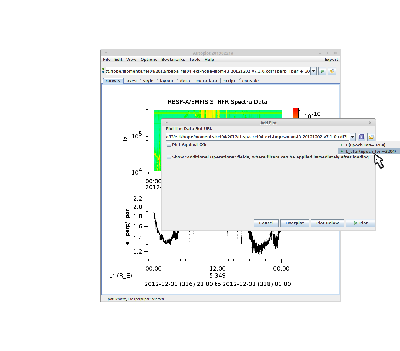
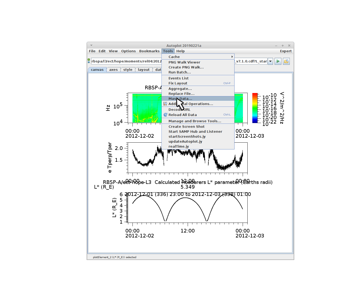
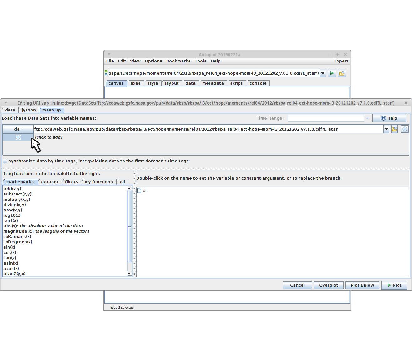
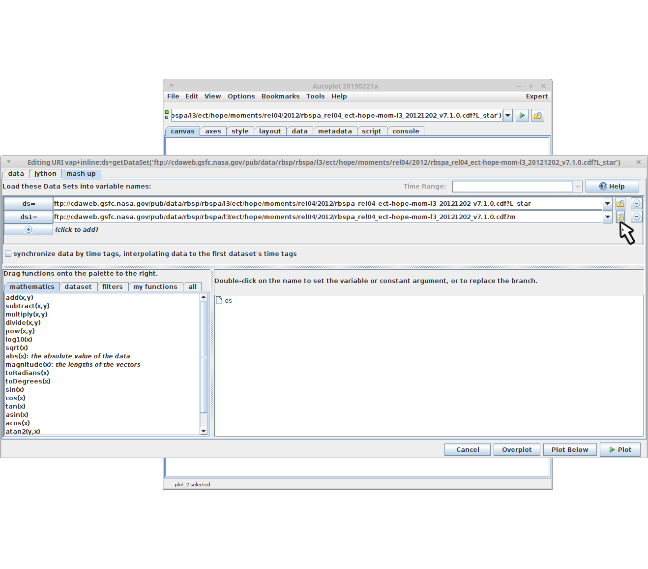
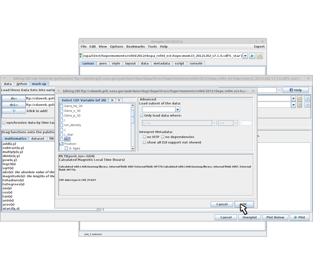
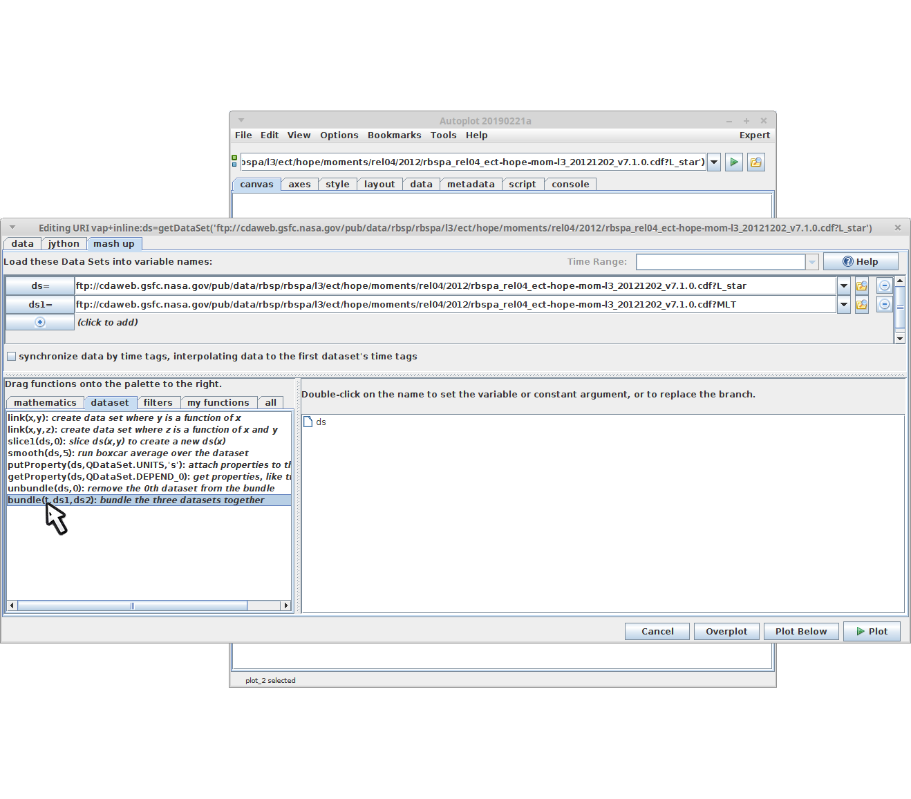
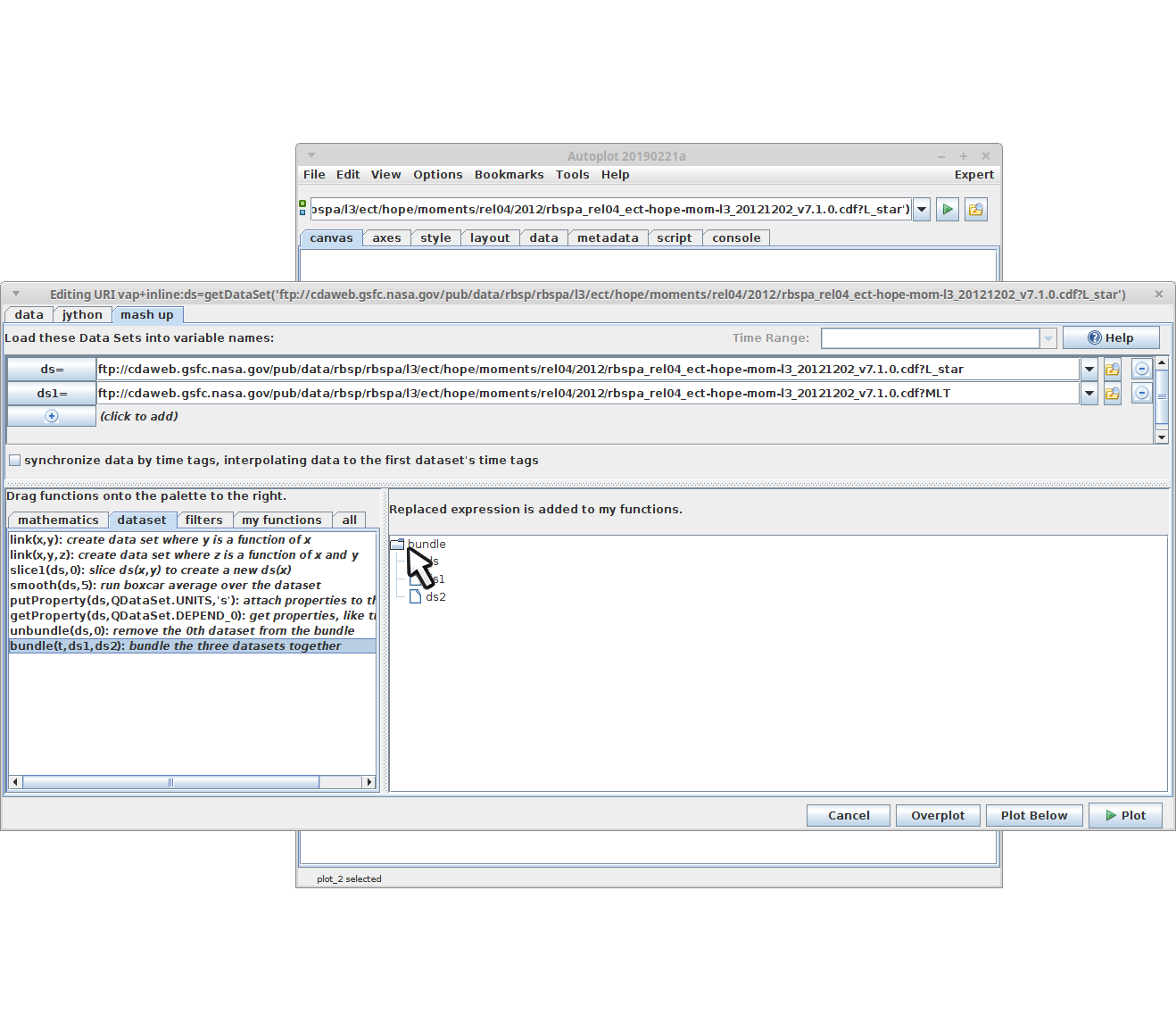
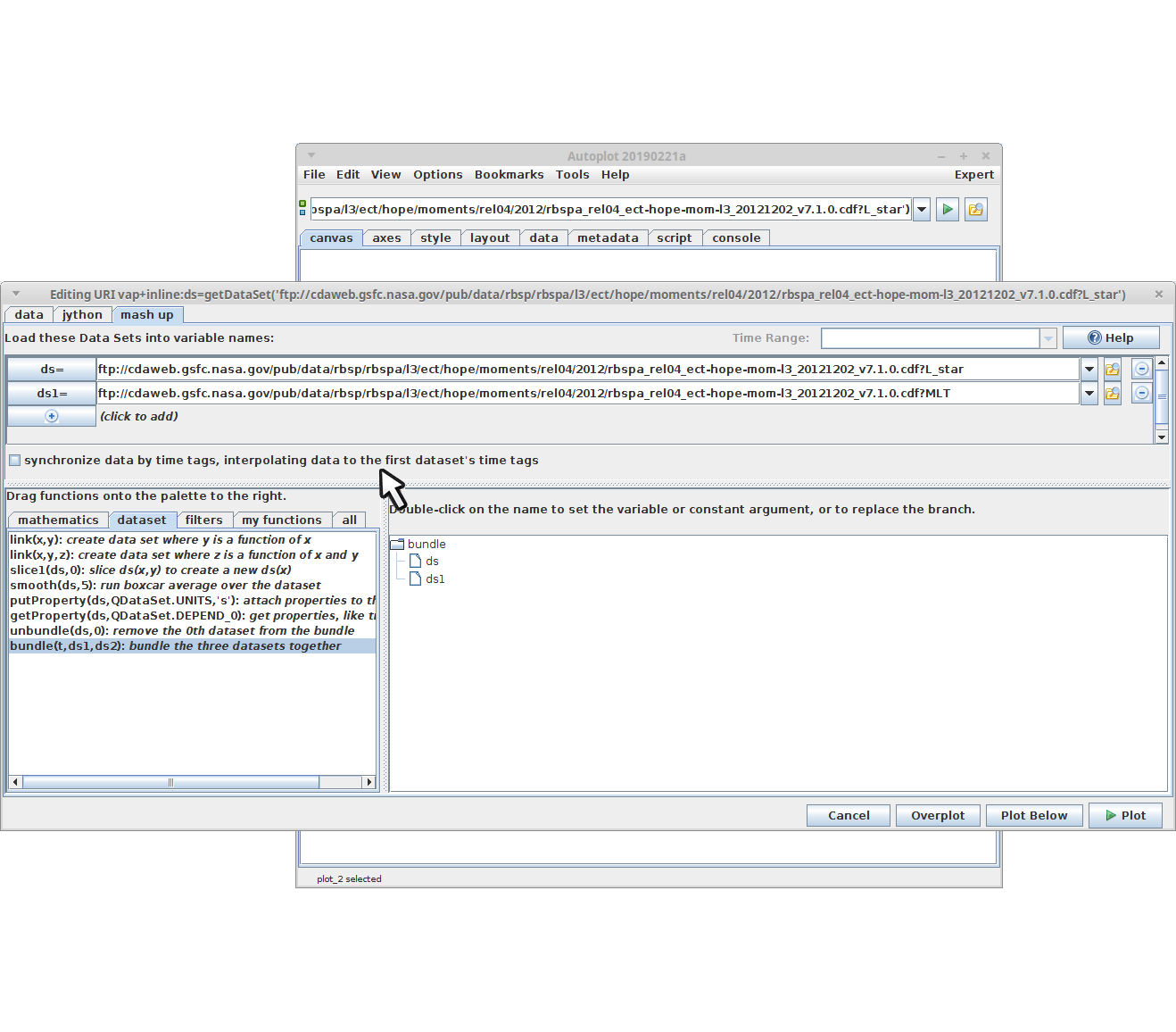
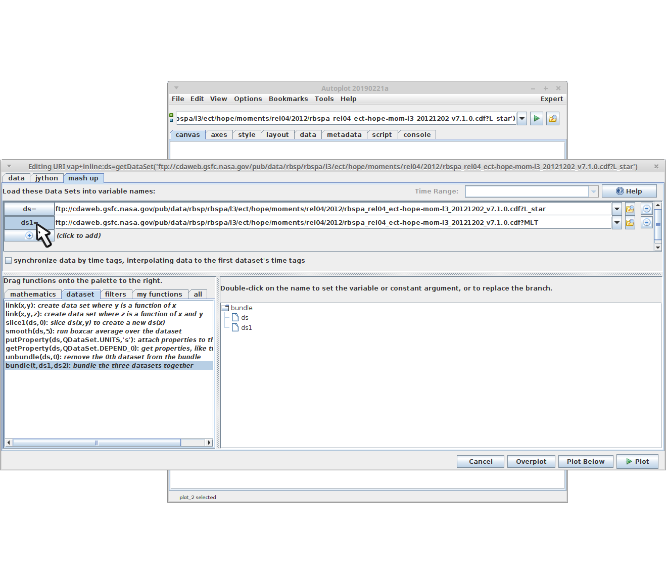
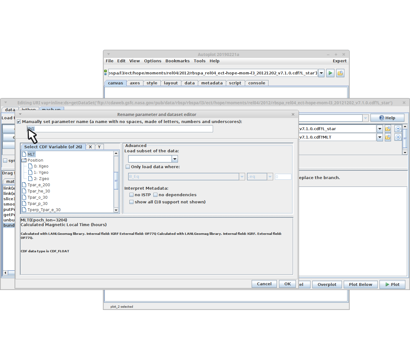
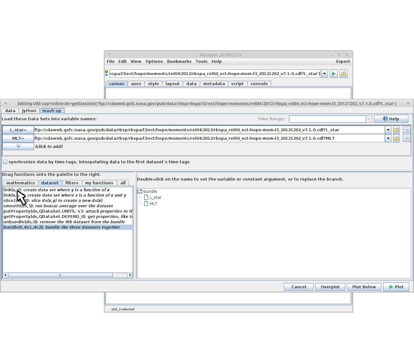
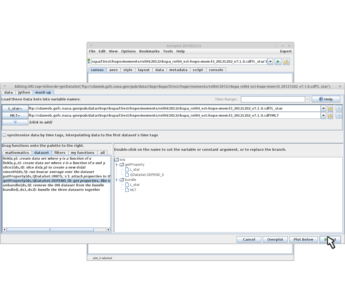
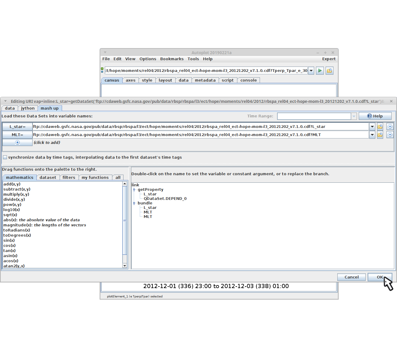
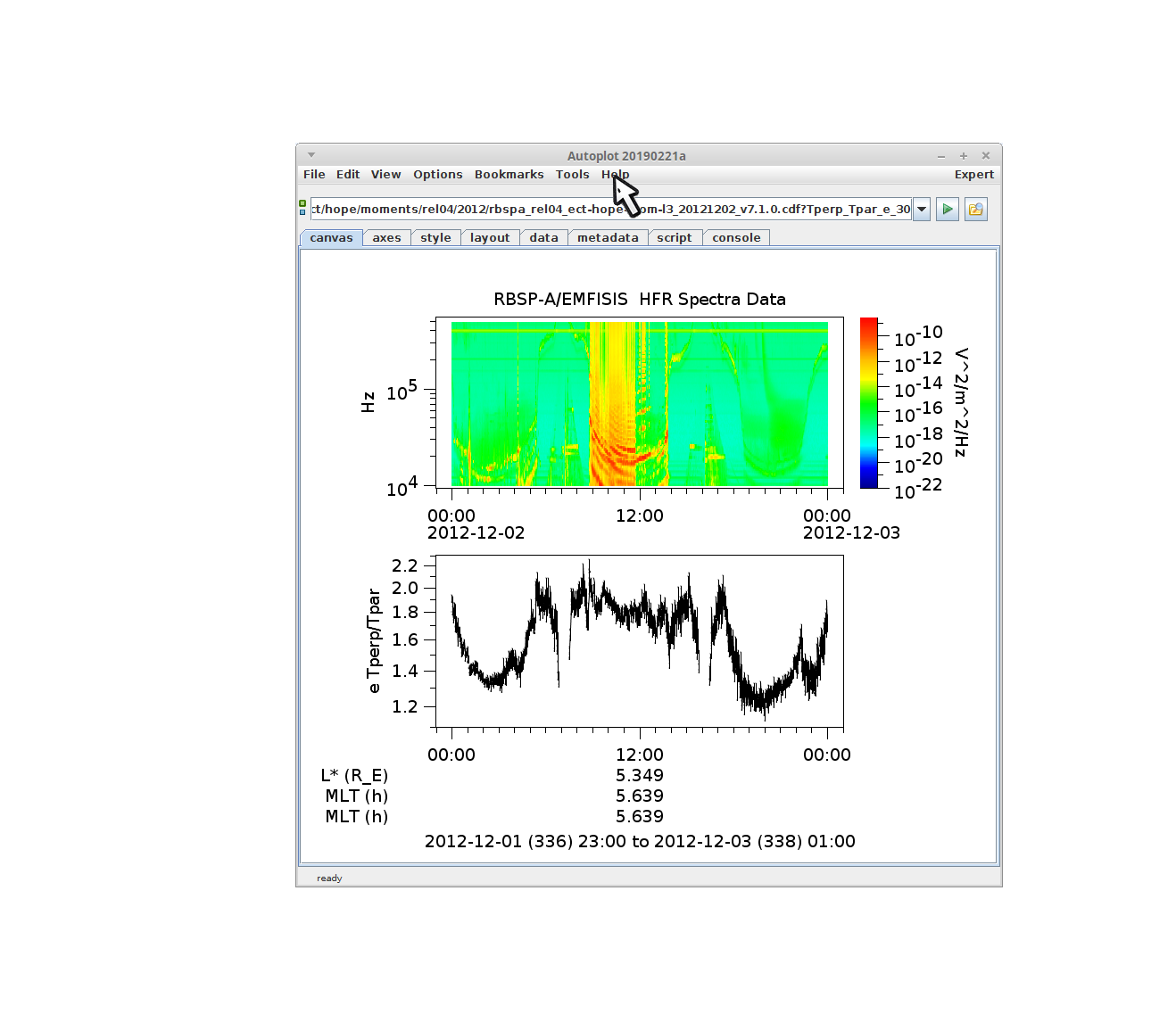
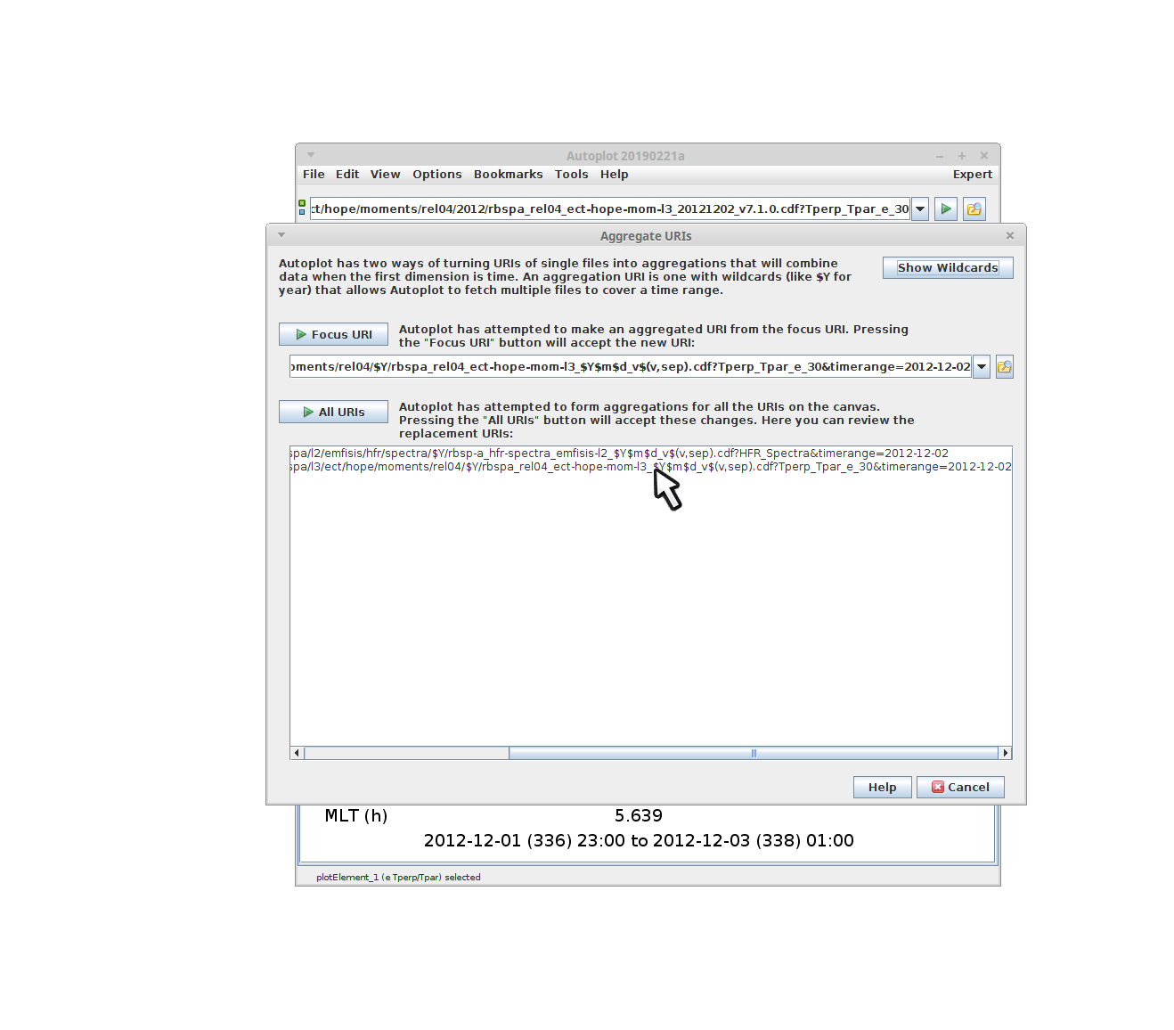
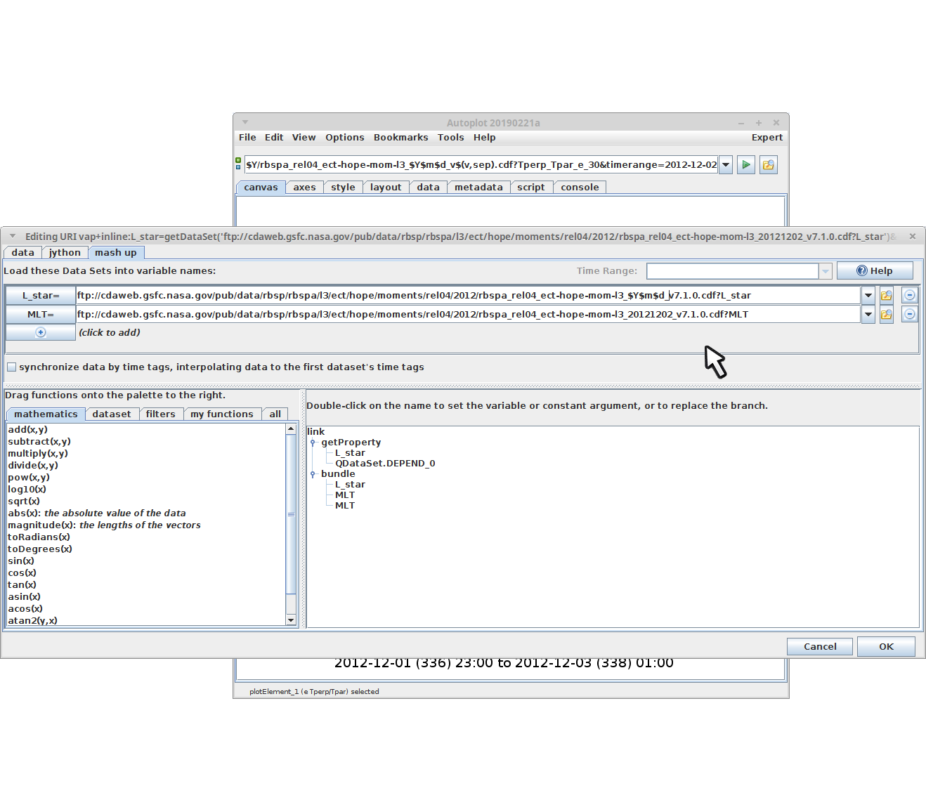
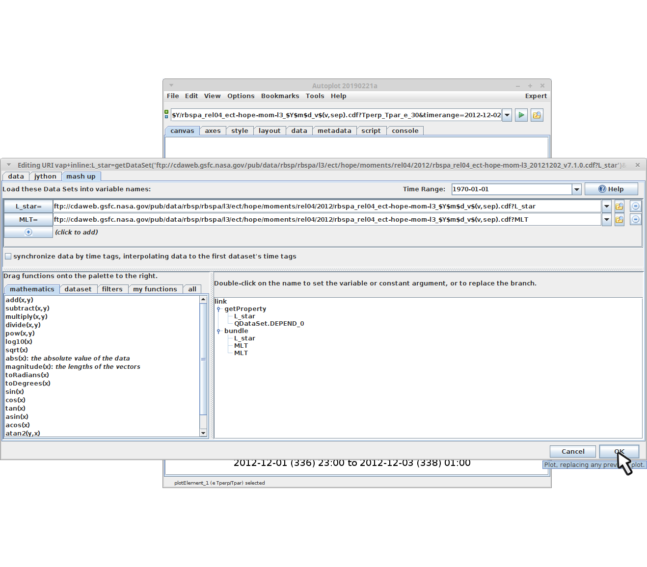
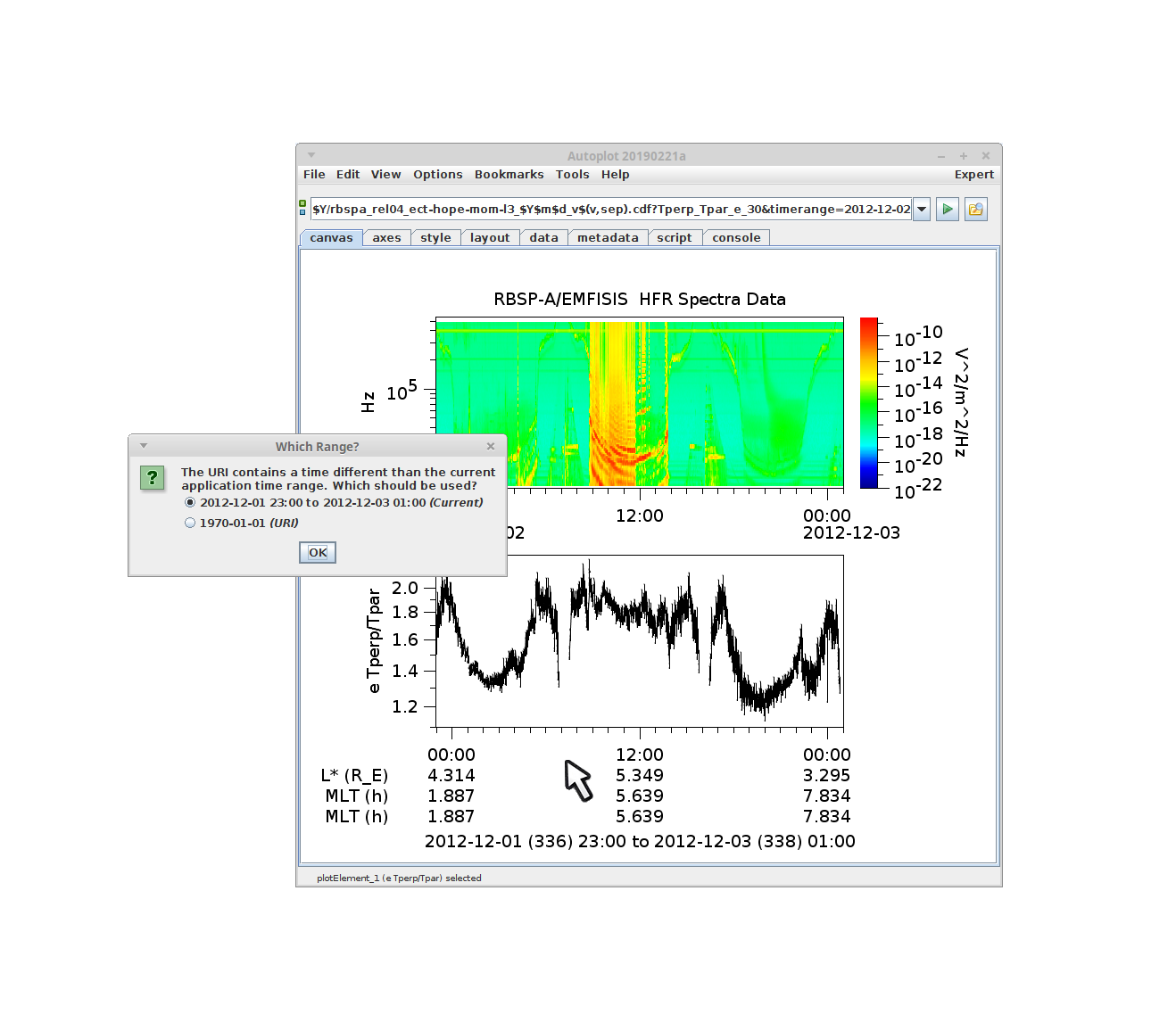
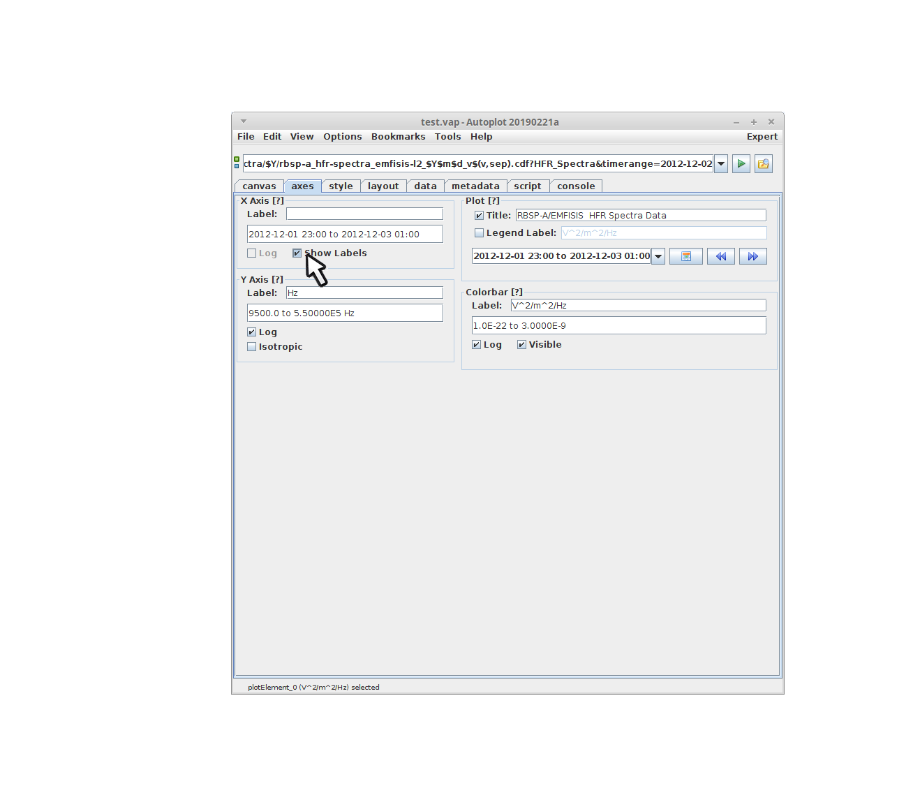
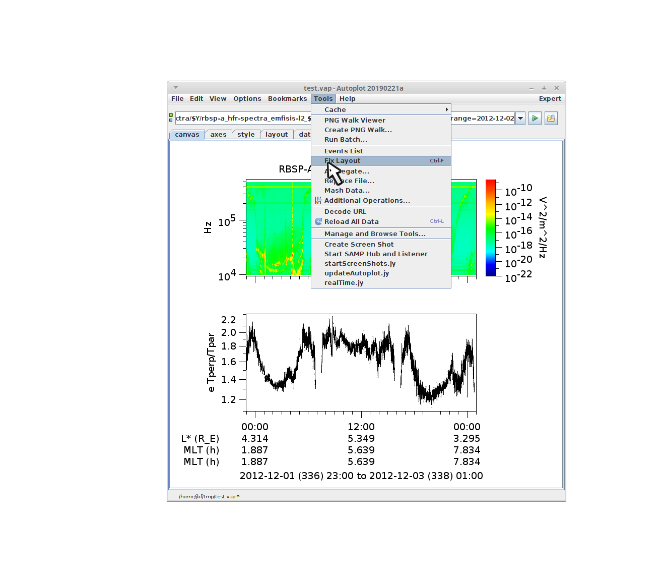
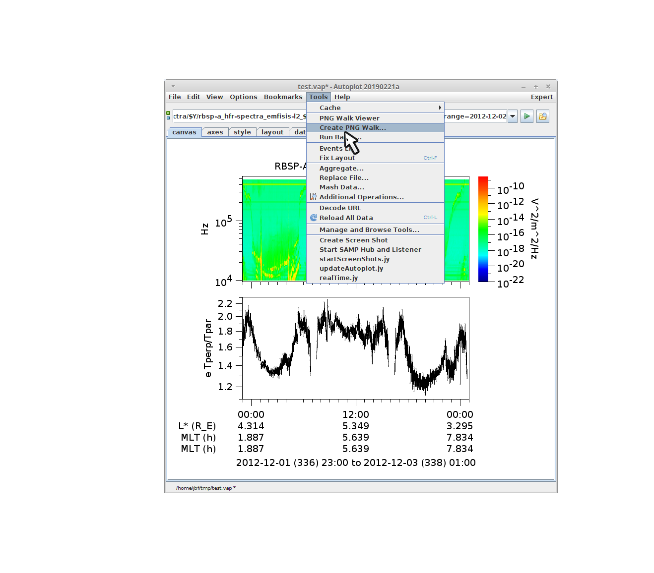
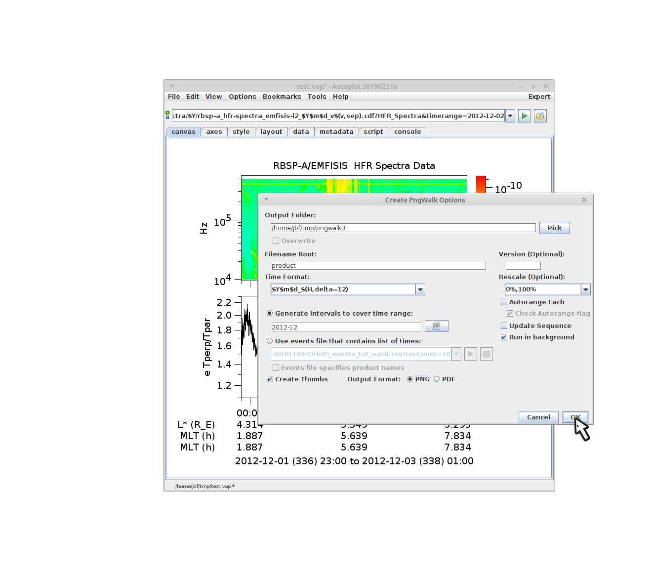
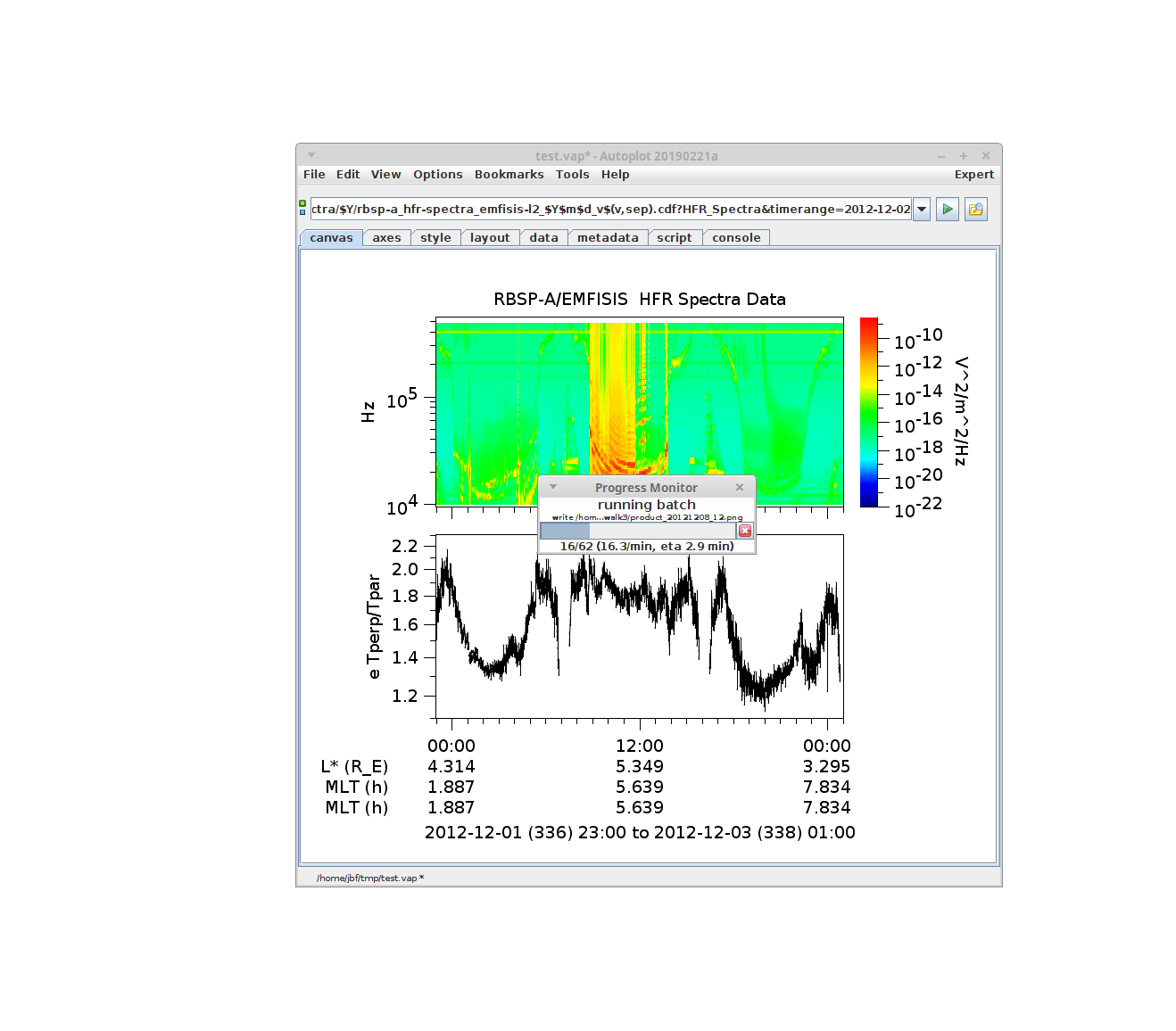
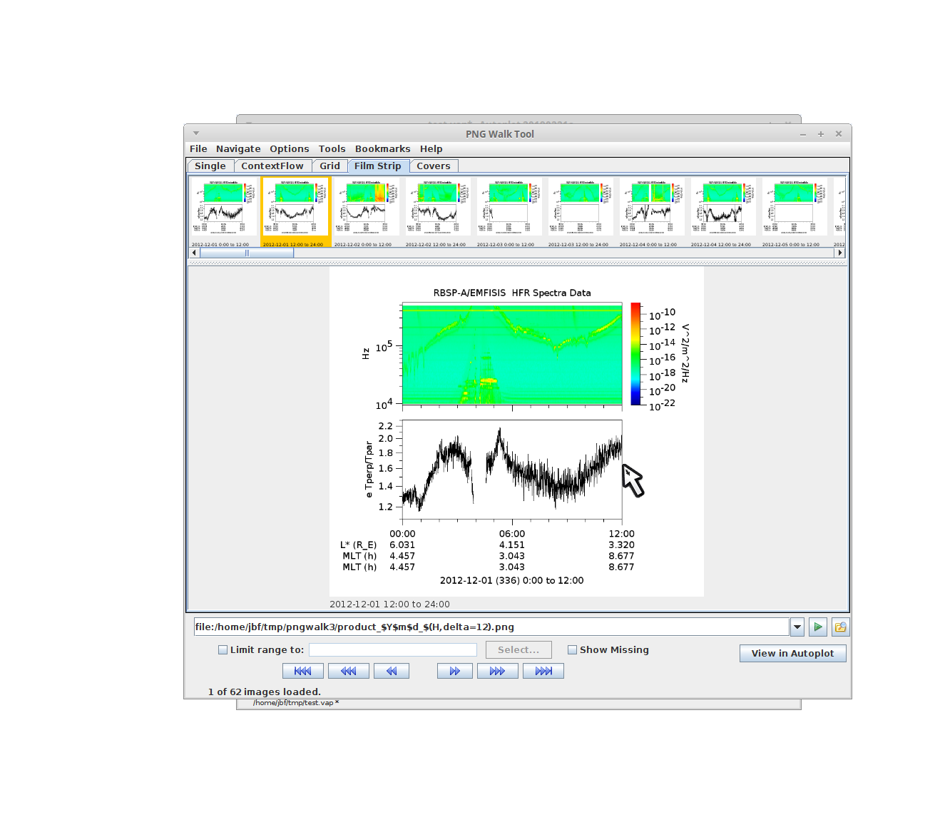
Copy and past the first URI.

Enter the editor to verify. Press Plot.

First plot. Now we'll add a plot below.

File->Add Plot...

Copy and paste the second URI.

When we verify it, we notice that a 0 was clipped from the URI. Select the proper variable.

"OK" to accept the variable.

"Plot below" to add the second plot.

The second plot is added. Note the title collides with the x axis label.

Turn off the bottom plot's title.

Now we'll add the ephemeris ticks. Copy the URI of the bottom plot. This CDF file also contains the some useful ephemeris.

Right-click on the xaxis and select "add additional ticks from..."

A dialog comes up, and we paste in the URI.

Re-enter the cdf URI editor, where we'll find ephemeris.

Select "L_star" and OK.

And OK the URI to add the one ephemeris line to the ticks.

Note there's no data at the two midnights. This is because it would have to extrapolate a little more than we're comfortable with.

To get multiple ticks, we have to use the mash-up tool. It's easiest to do this with a third plot so we can see what we are doing.

Select L star again and we'll plot it below. Note that tab-completions here show the parameters which start with L.

We've added the plot. We're going to delete it, so don't worry about the labels colliding.

Enter tools->Mash Data... to see how we can create a new URI which combines all the data.

The mash-up tool lets us create new datasets without all the effort of a full .jyds script. Click plus to add a second data set.

Enter a URI for the second dataset, and enter the editor.

select MLT

Select "bundle" on the dataset tab, and drag it over to the scratchpad.

drop on to the scratch pad. This is a tree of operations forming the new dataset.

Before we go further we can rename the variables to keep them straight.

Click on the label to reset the name.

Check "manual" and reset the name,

We need to do one more thing, to add timetags to the data. For this we use "link".

We get the DEPEND_0 from L_star and link those timetags to our bundle.

Unfortunately this doesn't work, because Autoplot thinks we want to look at a scatter plot instead of two line plots. This is because we need to have at least three things bundled.

A lot of things have happened, mostly where I was experimenting. But here I have three quantities plotted. Note I've moved the URI from our third plot to the ticks on the x-axis.

Okay, now we need to aggregate everything, so that we can run the pngwalk. Tools->Aggregate helps with this.

On the bottem panel, these are new URIs proposed. The "All URIs" button accepts these.

The data reloads using the aggregation. Note there is no data before and after midnight...

...and now there is. However the ticks are not using an aggregation, and we need to do those by hand.

Here we change them by hand.

Note the mash-up tool recognizes the aggregation and now "time range" is enabled.

It double-checks to make sure we want to use the same time as the other plots.

Note we have ticks at midnight now too. Our .vap is just about done and we'll save it.

Let's turn off the xaxis labels on the top plot too.

And run tools->fix layout.

Now for the PNGWalk.

Set up the PNGWalk to run.

To run the month takes a little while over a slower home connection.

But it eventually finishes and we can scroll around the pngwalk quickly.